Both of the derivative notations described in Section 6.2 distinguish between dependent quantities (\(f(x)\) or \(y\)) and the independent variable (\(x\)). However, in the real world one doesn’t always know in advance which variables are independent. We therefore go one step further, and express derivatives in terms of differentials.
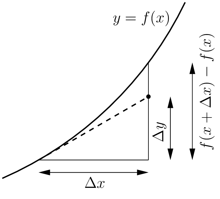
Figure6.1.Linear approximation using the tangent line.
The tangent line to the graph of \(y=f(x)\) at the point (\(x_0\text{,}\)\(y_0\)) is given by
\begin{equation}
y-y_0 = m \left( x-x_0 \right)\tag{6.4.1}
\end{equation}
where the slope \(m\) is of course just the derivative \(\frac{df}{dx} \big|_{x=x_0}\text{.}\) It is tempting to rewrite the equation of the tangent line as
\begin{equation}
\Delta y = \frac{df}{dx} \Delta x\tag{6.4.2}
\end{equation}
which is also used for linear approximation in the form
where the differential \(df\) can be interpreted as the corresponding small change in \(f\text{.}\)
The intuitive idea behind differentials is to consider the small quantities “\(dy\)” and “\(dx\)” separately, with the derivative \(\frac{dy}{dx}\) denoting their relative rate of change. So rather than either of the traditional expressions for derivatives (see Section 6.2), if \(y=x^2\) we write
\begin{equation}
dy = 2x\,dx .\tag{6.4.5}
\end{equation}
More generally, if \(y\) is any function of \(x\text{,}\) then the derivative\(\frac{dy}{dx}\) relates the differentials\(dy\) and \(dx\) via
\begin{equation}
dy = \frac{dy}{dx} dx .\tag{6.4.6}
\end{equation}
You can safely think of (6.4.5) as a sufficiently small quantity, or as the numerator of Leibniz notation, or as shorthand for a limit argument, or in terms of differential forms, or nonstandard analysis, or ...; it doesn’t matter, they all give the same equations.