Skip to main content
Contents Index Dark Mode Prev Up Next \(\newcommand{\vf}[1]{\mathbf{\boldsymbol{\vec{#1}}}}
\renewcommand{\Hat}[1]{\mathbf{\boldsymbol{\hat{#1}}}}
\let\VF=\vf
\let\HAT=\Hat
\newcommand{\Prime}{{}\kern0.5pt'}
\newcommand{\PARTIAL}[2]{{\partial^2#1\over\partial#2^2}}
\newcommand{\Partial}[2]{{\partial#1\over\partial#2}}
\newcommand{\tr}{{\mathrm tr}}
\newcommand{\CC}{{\mathbb C}}
\newcommand{\HH}{{\mathbb H}}
\newcommand{\KK}{{\mathbb K}}
\newcommand{\RR}{{\mathbb R}}
\newcommand{\HR}{{}^*{\mathbb R}}
\renewcommand{\AA}{\vf{A}}
\newcommand{\BB}{\vf{B}}
\newcommand{\CCv}{\vf{C}}
\newcommand{\EE}{\vf{E}}
\newcommand{\FF}{\vf{F}}
\newcommand{\GG}{\vf{G}}
\newcommand{\HHv}{\vf{H}}
\newcommand{\II}{\vf{I}}
\newcommand{\JJ}{\vf{J}}
\newcommand{\KKv}{\vf{Kv}}
\renewcommand{\SS}{\vf{S}}
\renewcommand{\aa}{\VF{a}}
\newcommand{\bb}{\VF{b}}
\newcommand{\ee}{\VF{e}}
\newcommand{\gv}{\VF{g}}
\newcommand{\iv}{\vf{imath}}
\newcommand{\rr}{\VF{r}}
\newcommand{\rrp}{\rr\Prime}
\newcommand{\uu}{\VF{u}}
\newcommand{\vv}{\VF{v}}
\newcommand{\ww}{\VF{w}}
\newcommand{\grad}{\vf{\nabla}}
\newcommand{\zero}{\vf{0}}
\newcommand{\Ihat}{\Hat I}
\newcommand{\Jhat}{\Hat J}
\newcommand{\nn}{\Hat n}
\newcommand{\NN}{\Hat N}
\newcommand{\TT}{\Hat T}
\newcommand{\ihat}{\Hat\imath}
\newcommand{\jhat}{\Hat\jmath}
\newcommand{\khat}{\Hat k}
\newcommand{\nhat}{\Hat n}
\newcommand{\rhat}{\HAT r}
\newcommand{\shat}{\HAT s}
\newcommand{\xhat}{\Hat x}
\newcommand{\yhat}{\Hat y}
\newcommand{\zhat}{\Hat z}
\newcommand{\that}{\Hat\theta}
\newcommand{\phat}{\Hat\phi}
\newcommand{\LL}{\mathcal{L}}
\newcommand{\DD}[1]{D_{\textrm{$#1$}}}
\newcommand{\bra}[1]{\langle#1|}
\newcommand{\ket}[1]{|#1\rangle}
\newcommand{\braket}[2]{\langle#1|#2\rangle}
\newcommand{\LargeMath}[1]{\hbox{\large$#1$}}
\newcommand{\INT}{\LargeMath{\int}}
\newcommand{\OINT}{\LargeMath{\oint}}
\newcommand{\LINT}{\mathop{\INT}\limits_C}
\newcommand{\Int}{\int\limits}
\newcommand{\dint}{\mathchoice{\int\!\!\!\int}{\int\!\!\int}{}{}}
\newcommand{\tint}{\int\!\!\!\int\!\!\!\int}
\newcommand{\DInt}[1]{\int\!\!\!\!\int\limits_{#1~~}}
\newcommand{\TInt}[1]{\int\!\!\!\int\limits_{#1}\!\!\!\int}
\newcommand{\Bint}{\TInt{B}}
\newcommand{\Dint}{\DInt{D}}
\newcommand{\Eint}{\TInt{E}}
\newcommand{\Lint}{\int\limits_C}
\newcommand{\Oint}{\oint\limits_C}
\newcommand{\Rint}{\DInt{R}}
\newcommand{\Sint}{\int\limits_S}
\newcommand{\Item}{\smallskip\item{$\bullet$}}
\newcommand{\LeftB}{\vector(-1,-2){25}}
\newcommand{\RightB}{\vector(1,-2){25}}
\newcommand{\DownB}{\vector(0,-1){60}}
\newcommand{\DLeft}{\vector(-1,-1){60}}
\newcommand{\DRight}{\vector(1,-1){60}}
\newcommand{\Left}{\vector(-1,-1){50}}
\newcommand{\Down}{\vector(0,-1){50}}
\newcommand{\Right}{\vector(1,-1){50}}
\newcommand{\ILeft}{\vector(1,1){50}}
\newcommand{\IRight}{\vector(-1,1){50}}
\newcommand{\Partials}[3]
{\displaystyle{\partial^2#1\over\partial#2\,\partial#3}}
\newcommand{\Jacobian}[4]{\frac{\partial(#1,#2)}{\partial(#3,#4)}}
\newcommand{\JACOBIAN}[6]{\frac{\partial(#1,#2,#3)}{\partial(#4,#5,#6)}}
\newcommand{\LLv}{\vf{L}}
\newcommand{\OOb}{\boldsymbol{O}}
\newcommand{\PPv}{\vf{P}_\text{cm}}
\newcommand{\RRv}{\vf{R}_\text{cm}}
\newcommand{\ff}{\vf{f}}
\newcommand{\pp}{\vf{p}}
\newcommand{\tauv}{\vf{\tau}}
\newcommand{\Lap}{\nabla^2}
\newcommand{\Hop}{H_\text{op}}
\newcommand{\Lop}{L_\text{op}}
\newcommand{\Hhat}{\hat{H}}
\newcommand{\Lhat}{\hat{L}}
\newcommand{\defeq}{\overset{\rm def}{=}}
\newcommand{\absm}{\vert m\vert}
\newcommand{\ii}{\ihat}
\newcommand{\jj}{\jhat}
\newcommand{\kk}{\khat}
\newcommand{\dS}{dS}
\newcommand{\dA}{dA}
\newcommand{\dV}{d\tau}
\renewcommand{\ii}{\xhat}
\renewcommand{\jj}{\yhat}
\renewcommand{\kk}{\zhat}
\newcommand{\lt}{<}
\newcommand{\gt}{>}
\newcommand{\amp}{&}
\definecolor{fillinmathshade}{gray}{0.9}
\newcommand{\fillinmath}[1]{\mathchoice{\colorbox{fillinmathshade}{$\displaystyle \phantom{\,#1\,}$}}{\colorbox{fillinmathshade}{$\textstyle \phantom{\,#1\,}$}}{\colorbox{fillinmathshade}{$\scriptstyle \phantom{\,#1\,}$}}{\colorbox{fillinmathshade}{$\scriptscriptstyle\phantom{\,#1\,}$}}}
\)
Section 17.4 The Dirac Delta Function
Definition 17.12 . The Dirac Delta Function.
Because the delta function has one point at which its value is infinite, it is not technically a function; it is a mathematical entity called a “distribution”, which is well defined only when it appears under an integral sign, as in
(17.4.2) .
The
Dirac delta function \(\delta(x)\) has has the following defining properties:
\begin{equation}
\delta(x)
= \begin{cases}
0\quad \amp x\not= 0\\
\infty\quad\amp x=0
\end{cases}\tag{17.4.1}
\end{equation}
\begin{equation}
\int_b^c \delta(x)\, dx = 1 \qquad\qquad b\lt 0\lt c\tag{17.4.2}
\end{equation}
\begin{equation}
x\,\delta(x) \equiv 0\text{.}\tag{17.4.3}
\end{equation}
Example 17.13 . Using the Dirac Delta Function in an Integral.
The properties of the delta function allow us to compute
\begin{align*}
\int_{-\infty}^{\infty} f(x)\,\delta(x) \,dx
\amp = \int_{-\infty}^{\infty} f(0)\,\delta(x) \,dx\\
\amp = f(0) \int_{-\infty}^{\infty} \delta(x) \,dx\\
\amp = f(0)
\end{align*}
(In the first equality, it is safe to replace the function \(f(x)\) with its value \(f(0)\) at \(x=0\) since everywhere else the delta function forces the integrand to be zero. For more details, see the visualization below.) We see that the Dirac delta function inside an integral picks out the value of the rest of the integrand at the point where the delta function is infinite.
We can shift the spike in the delta function as usual, obtaining \(\delta(x-a)\text{.}\) This shifted delta function satisfies
\begin{equation}
\int_{-\infty}^{\infty} f(x)\,\delta(x-a) \,dx
= f(a)\tag{17.4.4}
\end{equation}
To Remember. The Dirac delta function can be used inside an integral to pick out the value of a function at any desired point. This behaviour is the continuous analogue of a Kronecker delta, which can be used inside a sum to pick out a single term in the sum, for a more detailed comparison, see
Section 17.6 .
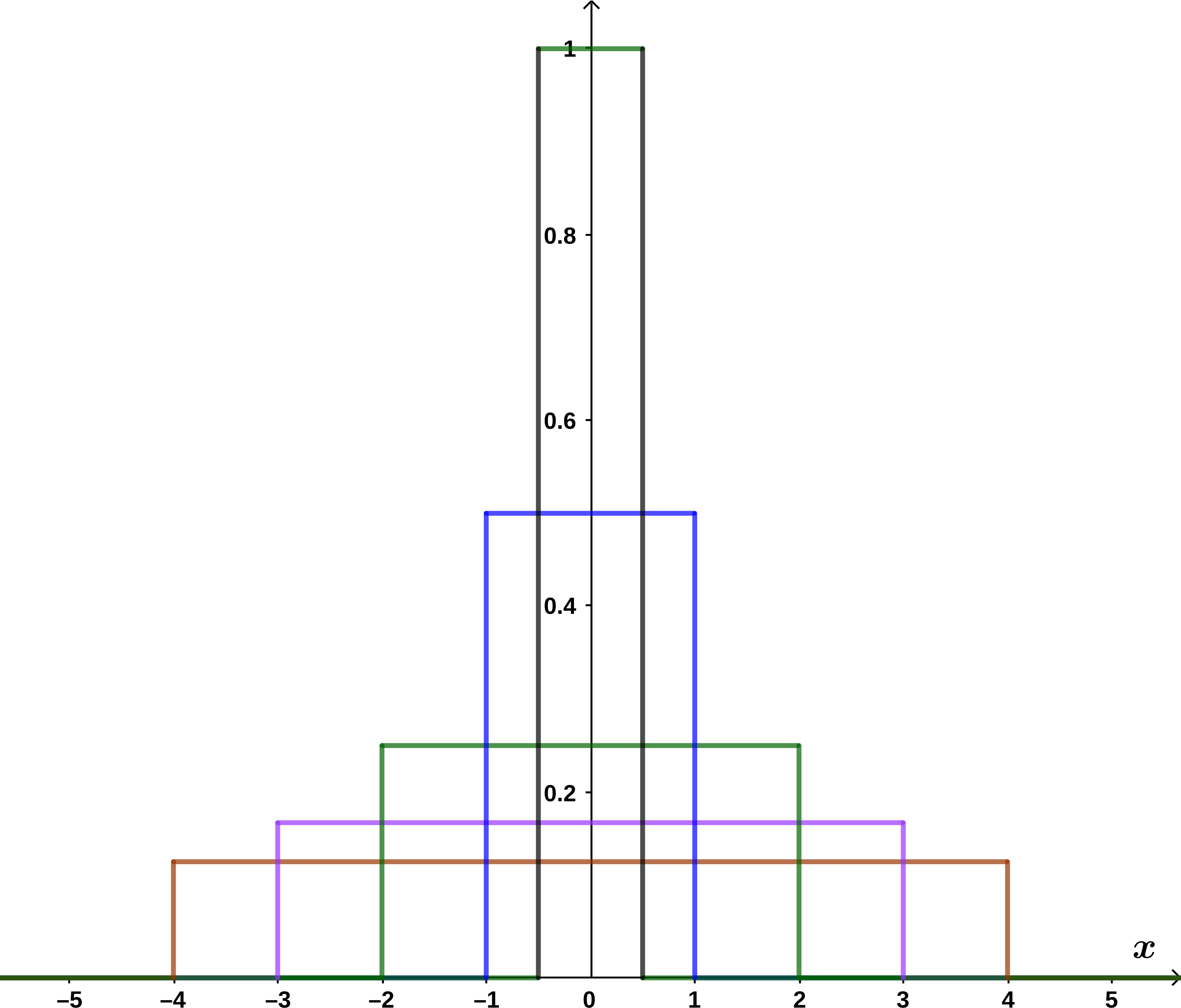
Visualization of the Delta Function. To understand why the delta function under an integral sign picks out a particular value of the integrand, it may help to think of the delta function as the limit of a sequence of steps
\(\delta_{\epsilon}(x)\text{,}\) Each step is narrower (width
\(2\epsilon\) ) and higher (height
\(1/(2\epsilon)\) ) than the previous step, such that the area under each step is always one; see Figure
Figure 17.14 .
Figure 17.14. The function \(\delta(x)\) can be approximated by a series of steps that get progressively thinner and higher in such a way that the area under the curve is always equal to one.
Then
\begin{equation}
\int_{-\infty}^{\infty} f(x)\, \delta_{\epsilon}(x-a)\, dx\tag{17.4.5}
\end{equation}
give the average value of \(f(x)\) on the interval determined by \(\epsilon\text{.}\) In the limit that \(\epsilon\) becomes infinitesimally small, then the peak becomes infinitely narrow and infinitely high in just the right way to pick out the value of the function at \(x=a\text{.}\)